











When pg_stat_statements flags a query as a top consumer, EXPLAIN ANALYZE is the operator’s ground truth. It shows what the executor did, node by node, buffer by buffer. Misreading the output leads to useless indexes and production changes that make performance worse.
This guide covers the mechanics that matter in production: how actual time accumulates through the node tree, why estimated rows diverge from reality, when buffer counts reveal cache misses versus disk reads, and how artifacts like the loops multiplier hide expensive nodes. It is a field manual for deciding, in the next five minutes, whether the problem is a missing index, stale statistics, a bad plan choice, or something deeper.
What EXPLAIN ANALYZE is and why it matters
Plain EXPLAIN shows the planner’s cost model and row estimates. It does not run the query. EXPLAIN ANALYZE executes the statement and collects actual wall-clock timing, actual row counts, and, with the BUFFERS option, buffer access counts per node.
In production, estimates diverge from reality after bulk loads or on correlated columns. EXPLAIN (ANALYZE, BUFFERS) reveals cache efficiency and identifies whether a sequential scan hits disk or runs entirely in shared buffers.
How a query plan executes and reports
The executor runs a tree of nodes. Data flows from leaf scans through joins, sorts, and aggregates toward the root. Each node reports its own metrics, but time and rows accumulate upward through the tree.
The output is a depth-first traversal. A Hash Join node sits above its build and probe children. The parent’s actual time includes time spent in children plus time the parent spent hashing or comparing keys. The build side should be the smaller relation; if the planner misestimates which side is smaller, you will see the larger relation being hashed and spilling to disk.
flowchart TD
    A[Aggregate] --> B[Hash Join]
    B -->|build| C[Seq Scan]
    B -->|probe| D[Index Scan]
    C -->|reads| E[Buffer Cache]
    D -->|reads| E

    A -.->|reports total runtime| F[Metrics]
    B -.->|reports node time| F
    C -.->|reports rows and buffers| F
    D -.->|reports rows and loops| F
The actual time format actual time=0.023..12.345 means the first output row appeared at 0.023 ms and the last at 12.345 ms. The second number is the node’s contribution to total runtime. When a node shows loops=N, multiply both actual time and actual rows by N before comparing to siblings or to the parent total. Ignoring this multiplication is the most common EXPLAIN reading mistake.
Reading the output: what each field means
Cost versus actual time. Costs are planner units, not milliseconds. Use them to compare nodes inside one plan, not to predict wall-clock time across queries. Actual time is measured wall-clock time. A high-cost node with low actual time is not the problem; a low-cost node with high actual time is where the optimizer guessed wrong. When actual time diverges wildly from cost, suspect stale statistics or a plan forced by a setting like enable_nestloop.
Estimated versus actual rows. When estimated rows differ from actual rows by an order of magnitude, the planner used bad cardinality data. If actual rows are far larger than estimated, the planner may have chosen a nested loop instead of a hash join. If actual rows are far smaller, the planner may have built a large hash table or sort buffer for a tiny result set. This mismatch signals missing indexes, stale statistics, or a table recently bulk-loaded and not yet analyzed.
Buffers. With BUFFERS, scan nodes report shared hit and shared read. shared hit is a buffer cache read; shared read is a disk fetch. Significant shared read on a frequently accessed table means the working set does not fit in memory or a sequential scan is bypassing indexes. shared read on a small lookup table that should be cached is a strong signal of a missing index or bloated pages. Healthy OLTP primaries usually keep cache hit ratio above 99%, so high shared read deserves attention. Nodes that modify data also report shared dirtied and shared written, which indicate writeback pressure.
Planning versus execution time. The summary line separates planning time from execution time. High planning time with low execution time indicates a complex query or too many join permutations. High execution time with low planning time indicates the chosen plan is inefficient.
Where misreadings happen in production
BitmapAnd and BitmapOr nodes always report actual rows = 0. This is an implementation artifact, not evidence that the bitmap found no rows. Do not use these row counts for cardinality checks.
Merge join row counts can exceed the inner relation size because duplicate keys cause rescans of the inner table. The reported row count is not ground truth for inner relation cardinality.
LIMIT clauses distort actual versus estimated comparisons. The planner estimates a full scan; actual values reflect early termination. A query with LIMIT 10 may show low actual time and high estimated cost. This is expected and does not indicate a bad plan.
Tables recently bulk-loaded, emptied, or smaller than autovacuum_analyze_threshold often have misleading estimates. Run ANALYZE manually after large data changes before trusting the plan.
EXPLAIN ANALYZE reads the system clock repeatedly, which slows execution measurably, especially for cheap queries. If you only need row counts and buffer data, use EXPLAIN (ANALYZE, BUFFERS, TIMING OFF). If you use auto_explain for passive monitoring, be aware that per-node timing adds overhead; disable it unless you are actively investigating a specific regression.
When to use EXPLAIN ANALYZE and when to avoid it
Use EXPLAIN (ANALYZE, BUFFERS, FORMAT JSON) when actively investigating a specific slow query and you need buffer counts and node-level timing. JSON format feeds visual tools such as pev2 or depesz, which help with complex plans.
Avoid running EXPLAIN ANALYZE on production write queries during peak load. It executes the query, so UPDATE or DELETE will modify data and add measurement overhead. For passive monitoring, rely on pg_stat_statements and auto_explain with conservative thresholds.
Signals to watch in production
| Signal | Why it matters | Warning sign |
|---|---|---|
| Seq Scan on large table with high actual time | Missing index or planner bypassing an index due to stale stats | Actual time exceeds 100 ms and actual rows exceed 10,000 |
| Nested Loop with loops greater than 1 and growing actual time | Fast iterations accumulate into dominant runtime | Loops exceed 1,000 and multiplied time exceeds parent node time |
| Shared read blocks far exceeding shared hit blocks | Working set is not cached; query is disk-bound | Shared read exceeds 10 percent of total buffers for OLTP queries |
| Actual rows far smaller than estimated rows | Planner overestimated selectivity; may have built large hash or sort structures | Estimated rows are 10 times larger than actual rows |
| Actual rows far larger than estimated rows | Planner underestimated result set; may have chosen nested loop over hash join | Actual rows are 10 times larger than estimated rows |
| High planning time in a simple query | Query structure or statistics forcing excessive planning work | Planning time exceeds execution time for routine queries |
How Netdata helps
Netdata collects PostgreSQL metrics that complement EXPLAIN ANALYZE and tell you when to reach for it.
- Query latency percentiles from
pg_stat_statementsexpose jumps in p99 execution time. A spike without a corresponding throughput change signals a plan regression or lock contention. - Cache hit ratio correlates with buffer counts from EXPLAIN output. A global drop in
blks_hit / (blks_hit + blks_read)confirms that queries showing highshared readare part of a systemic cache miss pattern. - Dead tuple ratio per table explains why scans return more actual rows than estimated. Rising dead tuples indicate stale statistics and approaching plan regressions.
- Lock wait events from
pg_stat_activityexplain why an efficient plan performs poorly under concurrency. - Autovacuum timestamps show whether
last_autovacuumis current. Stale timestamps mean blocked or missing vacuum runs degrade statistics and cause plan flapping. - Connection state breakdown tracks
active,idle, andidle in transactionsessions. Longidle in transactionsessions block vacuum and distort table statistics.
Related guides
- How PostgreSQL actually works in production: a mental model for operators
- PostgreSQL ALTER TABLE blocked: zero-downtime DDL patterns
- PostgreSQL autovacuum blocked by long-running transaction: detection and fix
- PostgreSQL autovacuum not running: detection, causes, and fixes
- PostgreSQL autovacuum tuning: per-table thresholds for high-churn workloads
- PostgreSQL blocking queries: finding the root blocker in a lock cascade
- PostgreSQL checkpoint storms: detection, causes, and tuning
- PostgreSQL: checkpoints are occurring too frequently – what to tune
- PostgreSQL connection exhaustion: detection, diagnosis, and prevention
- PostgreSQL connection refused: pg_hba, listen_addresses, and TCP diagnosis
- PostgreSQL: database is not accepting commands to avoid wraparound data loss
- PostgreSQL dead tuples piling up: why autovacuum can’t keep up